Shuttle sort
2021-12-11
Shuffle sort is an extension of bubble sort. It is used primarily as an educational tool.
Shuttle sort, also known as bidirectional bubble sort, cocktail sort, shaker sort, ripple sort, shuffle sort, shuttle sort or coktail sort, is an extension of bubble sort. It is used primarily as an educational tool.
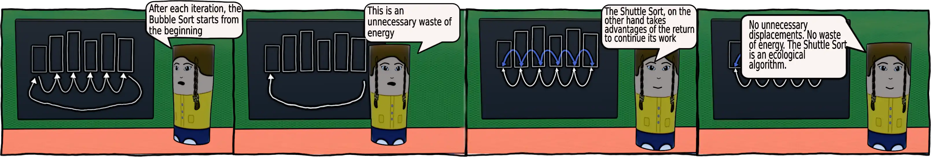
It tries to mitigate a defect of the bubble sort: the problem of rabbits and turtles. It’s a situation when a heavy bubble is placed at the end of the array. While the light bubbles (rabbits) are ascending rapidly, the heavy bubble (turtle) descends only one position per each iteration.
This algorithm will speed up the turtles by changing direction at each iteration. So with each change of direction, the “rabbits” become “turtles” and vice versa. It not only allows the larger elements to migrate quickly to the end of the list, but also allows the smaller elements to migrate faster to the beginning.
The animation below shows how the shuttle sort works :


Practical work
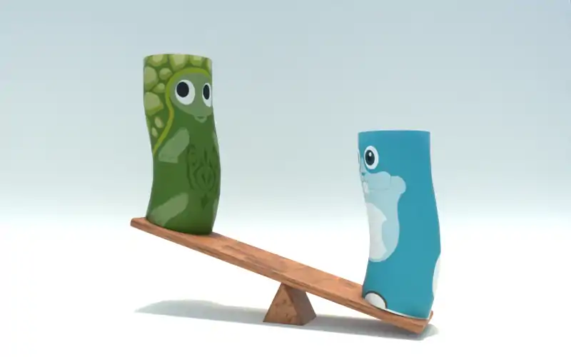
The mini-game below allows you to try to sort, in order of increasing weight, 5 barrels, with a Roberval scale to compare them. You can try to solve it with the shuttle sort method.
Variations
The most common version of this algorithm is composed of two nested loops.
void swap(int *a, int *b)
{
    int tmp = *a;
    *a = *b;
    *b = tmp;
}
void shakersort(int vect[], int size) {
    int step, current;
    for (step = 1; step <= size / 2; step++)
    {
        for (current = step - 1; current < size - step; current++)
            if (vect[current] > vect[current+1])
                swap(&vect[current], &vect[current + 1]);
        for (current = size - step - 1; current >= step; current--)
            if (vect[current] < vect[current-1])
                swap(&vect[current], &vect[current - 1]);
    }
}
But I prefer a version with a single loop and a change of direction. And, as for the bubble sort, you can stop after one iteration without permutation.
Complexity
The shaker sort does not add much to the bubble sort.
In the worst case, with data sorted in reverse, the successive runs of the table require (n2 - n) / 2 exchanges. For example, for a list of 10 items, it will take 45 comparisons and 45 exchanges [ (102 - 10) / 2 ]. The time complexity is therefore quadratic, of the order of O(n2).
When the initial order of the items to be sorted is random, it is considered that (n2 - 2*n) / 4 exchanges will be needed. The complexity will therefore also be O(n2).
In the best case, when the list is already sorted, it will take (n - 1) comparisons and no permutations. The time complexity is linear, in O(n).
In terms of space used (memory cost of the algorithm), the complexity of the shuttle sort is linear. It grows at the same speed as the number of input data. It is therefore O(n).
The animation below allows to verify, in an empirical way, this evolution of the number of operations according to the number of elements to sort.
| Data size | Comparisons | Swaps | Total |
|---|
To get a more concrete idea of the performance of this algorithm, suppose that you have to sort alphabetically the directory of the inhabitants of several large cities. And that the machine you have at your disposal can perform, say, ten million instructions per second . Here is the time that would be needed with this method:
| City | Population | Estimated sorting time |
|---|---|---|
| Paimpol (Brittany, France) | 7 172 | |
| Helsinki | 631 695 | |
| Denver | 705 576 | |
| Stockholm | 975 551 | |
| Berlin | 3 520 031 | |
| Nairobi | 4 734 881 | |
| Barcelona | 5 407 264 | |
| Rio | 6 718 000 | |
| Mosco | 12 655 050 | |
| Lagos | 22 829 561 | |
| Shanghai | 24 870 895 | |
| Seoul | 26 000 782 | |
| Manila | 28 644 207 | |
| Tokyo | 42 796 714 |